An stochastic jump process model for the 2017-2018 Influenza Season in Belgium

This tutorial is showcased in our software paper.

We’ll set up a simple stochastic model for Influenza in Belgium. First, we’ll expand the dynamics of the simple SIR model to account for additional disease charateristics of Influenza, and we’ll use the concept of dimensions to include four age groups in our model (called ‘age strata’). Opposed to the simple SIR tutorial, where changes in the number of social contacts were not considered, we’ll demonstrate how to use a time-dependent parameter function to include the effects of school closures during school holidays in our Influenza model. Finally, we’ll calibrate two of the model’s parameters to incrementally larger sets of incidence data and asses how the goodness-of-fit evolves with the amount of knowledge at our disposal. One of the calibrated model parameters will be a 1D vector, pySODM allows users to easily calibrate n-dimensional model parameters.

This tutorial introduces the following concepts,

1. Building a stochastic model and simulate it with Gillespie’s Tau-Leaping method

2. Extending an SIR model with age strata and using a social contact matrix

3. Calibrating an n-D model parameter to an n-D dataset

This tutorial can be replicated by running

python calibration.py

located in ~/tutorials/influenza_1718/. An environment containing the dependencies needed to run this tutorial is provided in ~/tutorial_env.yml.

Data

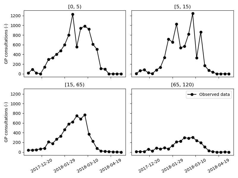
Data on the weekly incidence of visits to General Practictioners (GP) for Influenza-like illness (ILI) are made publically available by the Belgian Scientific Institute of Public Health (Sciensano). These data were retrieved from the “End of season” report on Influenza in Belgium (see data/raw/Influenza 2017-2018 End of Season_NL.pdf). Using Webplotdigitizer, the weekly number of GP visits in the different age groups were extracted (see data/raw/ILI_weekly_1718.csv). Then, the script data_conversion.py was used to convert the raw weekly incidence of Influenza cases in Belgium (per 100K inhabitats) during the 2017-2018 Influenza season into a better suited format. The week numbers in the raw dataset were replaced with the date of that week’s Thursday, as an approximation of the midpoint of the week. Further, the number of GP visits per 100K inhabitants was converted to the absolute number of GP visits. The formatted data are located in data/interim/ILI_weekly_100K.csv and data/interim/ILI_weekly_100K.csv.

The absolute weekly number of GP visits data are loaded in our calibration script ~/tutorials/influenza_1718/calibration.py as a pd.DataFrame with a pd.Multiindex. The weekly number of GP visits is divided by seven to approximate the daily incidence at the week’s midpoint (which we’ll use to calibrate our model). The time/date axis in the pd.DataFrame is obligatory. The other index names and values are the same as the model’s dimensions and coordinates. In this way, pySODM recognizes how model prediction and dataset must be aligned.

date        age_group
2017-12-01  (0, 5]        15.727305
            (5, 15]       13.240385
            (15, 65]     407.778693
            (65, 120]     32.379271
                            ...    
2018-05-11  (0, 5]         0.000000
            (5, 15]        0.000000
            (15, 65]       0.000000
            (65, 120]      0.000000
Name: CASES, Length: 96, dtype: float64

NOTE If we’d stratify our model further to include spatial patches, we could still calibrate the model to the DataFrame above. pySODM would, by default, sum over the model’s spatial axis to align the prediction with the data. This default summation over model axes not present in the data can be replaced with a user-defined function, see input argument aggregation_function of log_posterior_distribution.

Model dynamics, equations and parameters

We extend the classical Susceptible-Infectious-Recovered or SIR model of Kermack and McKendrick by making two changes to the compartmental structure. First, an exposed state (\(E\)) is added to account for the latent phase between the moment of infection and the onset of infectiousness. Second, the infectious state (\(I\)) is split in three parts. Individuals may experience infectiousness prior to symptom onset (\(I_{\text{pre}}\)). Then, after the onset of symptoms, not all infectious individuals will visit a GP and thus these individuals will not end up in the dataset. We include a state for individuals who are infectious but remain undetected (\(I_{\text{ud}}\)), and, we include a state for individuals who are infectious and go to a GP (\(I_{\text{d}}\)). All infectious individuals can transmit the disease. However, detected infectious individuals are assumed to only make 22% of the regular number of social contacts, corresponding to the fraction of contacts made at home.

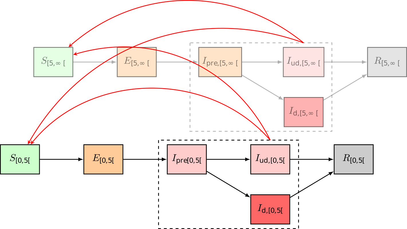
We’ll simulate these dynamics stochastically with Gillespie’s Tau-Leaping method. Instead of defining a differential equation for every model state, we need to define the rates of the six possible transitionings in the system,

\[\begin{split}\begin{cases} T^i &=& S^i + E^i + I_{\text{pre}}^i + I_{\text{ud}}^i + I_{\text{d}}^i + R^i, \nonumber\\ \mathcal{R}(S \rightarrow E)^i &=& \beta \sum_j N^{ij}(t) \dfrac{(I_{\text{pre}}^j + I_{\text{ud}}^j + 0.22 I_{\text{d}}^j)}{T^j}, \nonumber\\ \mathcal{R}(E \rightarrow I_{\text{pre}})^i &=& 1/\alpha, \nonumber \\ \mathcal{R}(I_{\text{pre}} \rightarrow I_{\text{ud}})^i &=& f_{\text{ud}}^i/\gamma, \nonumber \\ \mathcal{R}(I_{\text{pre}} \rightarrow I_{\text{d}})^i &=& (1-f_{\text{ud}}^i)/\gamma, \nonumber \\ \mathcal{R}(I_{\text{ud}} \rightarrow R)^i &=& 1/\delta, \nonumber \\ \mathcal{R}(I_d \rightarrow R)^i &=& 1/\delta, \end{cases}\end{split}\]

where the subscript \(i\) refers to the model’s age groups: \([0,5(, [5,15(, [15,65(,\text{ and } [65,120(\) years old. \(T\) denotes the total population, \(S\) denotes the number of individuals susceptible to the disease, \(E\) denotes the number of exposed individuals, \(I_{\text{pre}}\) denotes the number of presymptomatic infectious individuals, \(I_{\text{ud}}\) denotes the number of infectious but undetected individuals and \(I_{\text{d}}\) denotes the number of infectious individuals who visit the GP, \(R\) denotes the number of removed individuals, either through death or recovery. The model has six parameters,

• \(\alpha\): Duration of the latent phase, equal to one day.

• \(\beta\) : Per-contact chance of Influenza transmission. Calibrated.

• \(\gamma\) : Duration of pre-symptomatic infectiousness, equal to one day.

• \(\delta\) : Duration of infectiousness, equal to one day.

• \(N^{ij}\) : Square origin-destination matrix containing the number of social contacts in age group \(i\) with individuals from age group \(j\). Extracted from Socrates. Dataset: Hoang, Belgium, 2010. Physical contacts with a duration of 15+ minutes only. Integrated with contact duration.

• \(f_{\text{ud}}^i\) : Age-stratified fraction of undetected cases. Calibrated.

Assuming the aforementioned transition rates from a generic state \(X\) to a state \(Y\) in age group \(i\), denoted \(\mathcal{R}(X \rightarrow Y)^i\), are constant over the interval \([t,t+\tau]\), the probability of a transition from a generic state \(X\) to \(Y\) happening in the interval \([t,t+\tau]\) is exponentially distributed, mathematically,

\[\mathcal{P}(X \rightarrow Y)^i = 1 - e^{- \tau*\mathcal{R}(X \rightarrow Y)^i}.\]

The corresponding number of transitions \(X \rightarrow Y\) in age class \(i\) and between time \(t\) and \(t + \tau\) are then generated by drawing from a binomial distribution,

\[\mathcal{N}(X \rightarrow Y)^i = Binom(\mathcal{P}(X \rightarrow Y)^i, X^i).\]

The number of individuals in each of the compartments at time \(t + \tau\) is then given by,

\[\begin{split}\begin{cases} S^i(t+\tau) &=& S^i(t) - \mathcal{N}(S \rightarrow E)^i, \nonumber \\ E^i(t+\tau) &=& E^i(t) + \mathcal{N}(S \rightarrow E)^i - \mathcal{N}(E \rightarrow I_{\text{pre}})^i, \nonumber\\ I_{\text{pre}}^i(t+\tau) &=& I_{\text{pre}}^i(t) + \mathcal{N}(E \rightarrow I_{\text{pre}})^i - \mathcal{N}(I_{\text{pre}} \rightarrow I_{\text{ud}})^i - \mathcal{N}(I_{\text{pre}} \rightarrow I_{\text{d}})^i, \nonumber\\ I_{\text{ud}}^i(t+\tau) &=& I_{\text{ud}}^i(t) + \mathcal{N}(I_{\text{pre}} \rightarrow I_{\text{ud}})^i - \mathcal{N}(I_{\text{ud}} \rightarrow R)^i, \nonumber \\ I_{\text{d}}^i(t+\tau) &=& I_{\text{d}}^i(t) + \mathcal{N}(I_{\text{pre}} \rightarrow I_{\text{d}})^i - \mathcal{N}(I_d \rightarrow R)^i, \nonumber \\ R^i(t+\tau) &=& R^i(t) + \mathcal{N}(I_{\text{ud}} \rightarrow R)^i + \mathcal{N}(I_\text{d} \rightarrow R)^i. \end{cases}\end{split}\]

The daily number of GP visits (incidence) is computed as,

\[\begin{equation} I_{\text{d, inc}}^i(t+\tau) = \mathcal{N}(I_{\text{pre}} \rightarrow I_{\text{d}})^i. \end{equation}\]

We’ll match this state to the dataset. The basic reproduction number in age group \(i\) of the equivalent deterministic model can be computed using the next-generation matrix approach introduced by Diekmann et al.,

\[\begin{equation} R_0^i = \beta \big(\gamma + f_{\text{ud}}^i \delta + 0.22 (1-f_{\text{ud}})\delta\big) \sum_j N^{ij}, \end{equation}\]

and the population basic reproduction number is computed as the weighted average over all age groups using demographic data.

Coding it up

The model

Opposed to ODE models, where the user had to define an integrate() function to compute the values of the derivatives at time \(t\), the user will have to define two functions to setup an stochastic jump process model: 1) A function to compute the rates at time \(t\) named compute_rates(), and 2) A function to compute the values of the model states at time \(t+\tau\) named apply_transitionings(). As we did in the packed-bed continuous flow reactor tutorial, we’ll stratifiy the model into age groups by specifying a variable dimensions in our model declaration and we’ll implement the parameter \(f_a\) as a stratified parameter by specifying a variable stratified_parameters. As dimension name, we use the same name as the age dimension in the dataset: 'age_group'. The coordinates of the dimension will be defined later when the model is initialized, we’ll have to use the same coordinates as the dataset. As in the enzyme kinetics tutorial, we’ll group our model in a file called models.py to reduce the complexity of our calibration script. We introduce one additional state in the model, the incidence of new detected cases, I_m_inc, which we’ll use this state to match our data to.

from pySODM.models.base import JumpProcess

class JumpProcess_influenza_model(JumpProcess):
    """
    Simple stochastic SEIR model for influenza with undetected carriers
    """
    
    states = ['S','E','Ip','Iud','Id','R','Im_inc']
    parameters = ['alpha', 'beta', 'gamma', 'delta','N']
    stratified_parameters = ['f_ud']
    dimensions = ['age_group']

    @staticmethod
    def compute_rates(t, S, E, Ip, Iud, Id, R, Im_inc, alpha, beta, gamma, delta, N, f_ud):
        
        # Calculate total population
        T = S+E+Ip+Iud+Id+R
        # Compute rates per model state
        rates = {
            'S': [beta*np.matmul(N, (Ip+Iud+0.22*Id)/T),],
            'E': [1/alpha*np.ones(T.shape),],
            'Ip': [f_ud*(1/gamma), (1-f_ud)*(1/gamma)],
            'Iud': [(1/delta)*np.ones(T.shape),],
            'Id': [(1/delta)*np.ones(T.shape),],
        }
        
        return rates

    @staticmethod
    def apply_transitionings(t, tau, transitionings, S, E, Ip, Iud, Id, R, Im_inc, alpha, beta, gamma, delta, N, f_ud):

        S_new  = S - transitionings['S'][0]
        E_new = E + transitionings['S'][0] - transitionings['E'][0]
        Ip_new = Ip + transitionings['E'][0] - transitionings['Ip'][0] - transitionings['Ip'][1]
        Iud_new = Iud + transitionings['Ip'][0] - transitionings['Iud'][0]
        Id_new = Id + transitionings['Ip'][1] - transitionings['Id'][0]
        R_new = R + transitionings['Iud'][0] + transitionings['Id'][0]
        Im_inc_new = transitionings['Ip'][1]

        return S_new, E_new, Ip_new, Iud_new, Id_new, R_new, Im_inc_new

There are some formatting requirements to compute_rates() and apply_transitionings(), which are listed in the JumpProcess documentation.

The actual drawing of the transitionings is abstracted away from the user in the JumpProcess class. Two stochastic simulation algorithms are currently available. In this tutorial, we’ll use the Tau-Leaping method, where the value of tau is fixed and the number of transitionings in the interval t and t + \tau are drawn from a binomial distribution. This method is an approximation of the Stochastic Simulation Algorithm (SSA), where the time until the first transitioning tau is computed and only one transitioning can happen at every simulation step. However, as we aim to simulate a large number of individuals (11 million individuals), the time between transitionings becomes very small and the SSA becomes computationally too demanding. Good values for tau are typically found by balancing the use of computational resources against numerical stability.

Social contact function

The number of work and school contacts tends to change during school holidays and this has an effect on Influenza spread. We’ll thus use a time-dependent parameter function to vary the number of social contacts \(\mathbf{N}\) during the simulation. We’ll wrap our contact_function() in a class for the sake of user friendliness. The initialization of the class is used to store the contact matrices inside the dictionary \(\mathbf{N}\). The callable function __call__ is used to return the right contact matrix. The contact_function() is the actual pySODM-compatible time-dependent parameter function, which implements the social policies. We’ll add our TDPF to the models.py script.

class make_contact_matrix_function():

    def __init__(self, N):
        """
        Initialize the class by storing the dictionary of contacts

        Input
        =====

        N: dict
            Dictionary holding the contact matrices.
            Contains two levels. 1) holiday/no_holiday, 2) week/weekend
        """

        self.N = N

    def __call__(self, t, holiday=False):
        """
        A function to choose the appropriate contact matrix (holiday? weekend?)
        """

        # Choose between holiday/no_holiday
        if holiday:
            N = self.N['holiday']
        else:
            N = self.N['no_holiday']
        
        # Choose between weekday and weekendday
        if ((t.weekday() == 5) | (t.weekday() == 6)):
            return N['weekend']
        else:
            return N['week']

    # Define a pySODM compatible wrapper with the social policies
    def contact_function(self, t, states, param):
        """
        A pySODM compatible wrapper containing the social policies

        Input
        =====

        t: timestamp
            Current simulated date

        states: dict
            Dictionary containing model states at current time

        param: dict
            Dictionary containing all model parameters

        Output
        ======

        N: np.ndarray (4x4)
            Matrix of social contacts at time `t`

        """
        t = pd.to_datetime(t)

        if t <= pd.Timestamp('2017-10-30'):
            return self.__call__(t)
        # Winter holiday
        elif pd.Timestamp('2017-10-30') < t <= pd.Timestamp('2017-11-05'):
            return self.__call__(t, holiday=True)
        # Winter holiday --> Christmas holiday
        elif pd.Timestamp('2017-11-05') < t <= pd.Timestamp('2017-12-22'):
            return self.__call__(t)    
        # Christmas holiday
        elif pd.Timestamp('2017-12-22') < t <= pd.Timestamp('2018-01-07'):
            return self.__call__(t, holiday=True)
        # Christmas holiday --> Spring holiday
        elif pd.Timestamp('2018-01-07') < t <= pd.Timestamp('2018-02-12'):
            return self.__call__(t)
        #Spring holiday
        elif pd.Timestamp('2018-02-12') < t <= pd.Timestamp('2018-02-18'):
            return self.__call__(t, holiday=True)
        # Spring holiday --> Easter holiday
        elif pd.Timestamp('2018-02-18') < t <= pd.Timestamp('2018-04-02'):
            return self.__call__(t)
        # Easter holiday
        elif pd.Timestamp('2018-04-02') < t <= pd.Timestamp('2018-04-15'):
            return self.__call__(t, holiday=True)
        else:
            return self.__call__(t)

Initializing the model

Next, we’ll set the model up in our calibration script ~/tutorials/influenza_1718/calibration.py. We load the model and social contact function from models.py and initialize the contact matrix function using the social contact matrices (hardcoded in the example). Then, as always, we define the model parameters, initial states (obtained analytically so the differentials are zero at \(t=0\)) and coordinates. The coordinates for dimension age_groups must be the same as the dataset: pd.IntervalIndex.from_tuples([(0,5),(5,15),(15,65),(65,120)].

# Load model
from models import JumpProcess_influenza_model as influenza_model

# Load TDPF
from models import make_contact_matrix_function

# Hardcode the contact matrices
N_noholiday_week = ...
N_noholiday_weekend = ...
N_holiday_week = ...

# Construct a dictionary of contact matrices
N = {
    'holiday': {'week': N_holiday_week, 'weekend': N_noholiday_weekend},
    'no_holiday': {'week': N_noholiday_week, 'weekend': N_noholiday_weekend}
}

# Initialize contact function
from models import make_contact_matrix_function
contact_function = make_contact_matrix_function(N).contact_function

# Define model parameters
params={'alpha': 1, 'beta': 0.0174, 'gamma': 1, 'delta': 3,'f_ud': np.array([0.01, 0.64, 0.905, 0.60]), 'N': N['holiday']['week']}

# Define initial condition
init_states = {'S': list(initN.values),
              'E': list(np.rint((1/(1-params['f_ud']))*df_influenza.loc[start_calibration, slice(None)])),
              'Ip': list(np.rint((1/(1-params['f_ud']))*df_influenza.loc[start_calibration, slice(None)])),
              'Iud': list(np.rint((params['f_ud']/(1-params['f_ud']))*df_influenza.loc[start_calibration, slice(None)])),
              'Id': list(np.rint(df_influenza.loc[start_calibration, slice(None)])),
              'Im_inc': list(np.rint(df_influenza.loc[start_calibration, slice(None)]))}

# Define model coordinates
coordinates={'age_group': age_groups}

# Initialize model
model = influenza_model(init_states,params,coordinates,time_dependent_parameters={'N': contact_function})

Calibration

We aim to calibrate two model parameters: \(\beta\) and \(\mathbf{f_{ud}}\). However, \(\mathbf{f_{ud}}\) consists of four elements \(f_{ud}^i\), how does pySODM handle this?

As if nothing’s up,

if __name__ == '__main__':

    from pySODM.optimization.objective_functions import log_posterior_probability, ll_negative_binomial

    # Define dataset
    data=[df_influenza[start_date:end_calibration], ]
    states = ["Im_inc",]
    log_likelihood_fnc = [ll_negative_binomial,]
    log_likelihood_fnc_args = [4*[0.03,],]

    # Calibated parameters and bounds
    pars = ['beta', 'f_ud']
    labels = ['$\\beta$', '$f_{ud}$']
    bounds = [(1e-6,0.06), (0,0.99)]

    # Setup objective function (no priors --> uniform priors based on bounds)
    objective_function = log_posterior_probability(model, pars, bounds, data, states, log_likelihood_fnc, log_likelihood_fnc_args, labels=labels)

In the example above, bounds and labels of \(\mathbf{f_{ud}}\) are automatically expanded to the right size when the log posterior probability function is initialized. However, I have retained the possibility of supplying a bound and label per element of \(\mathbf{f_{ud}}\). Running the NM/PSO and MCMC optimizations happens in the same manner as the other tutorials.

Results and discussion

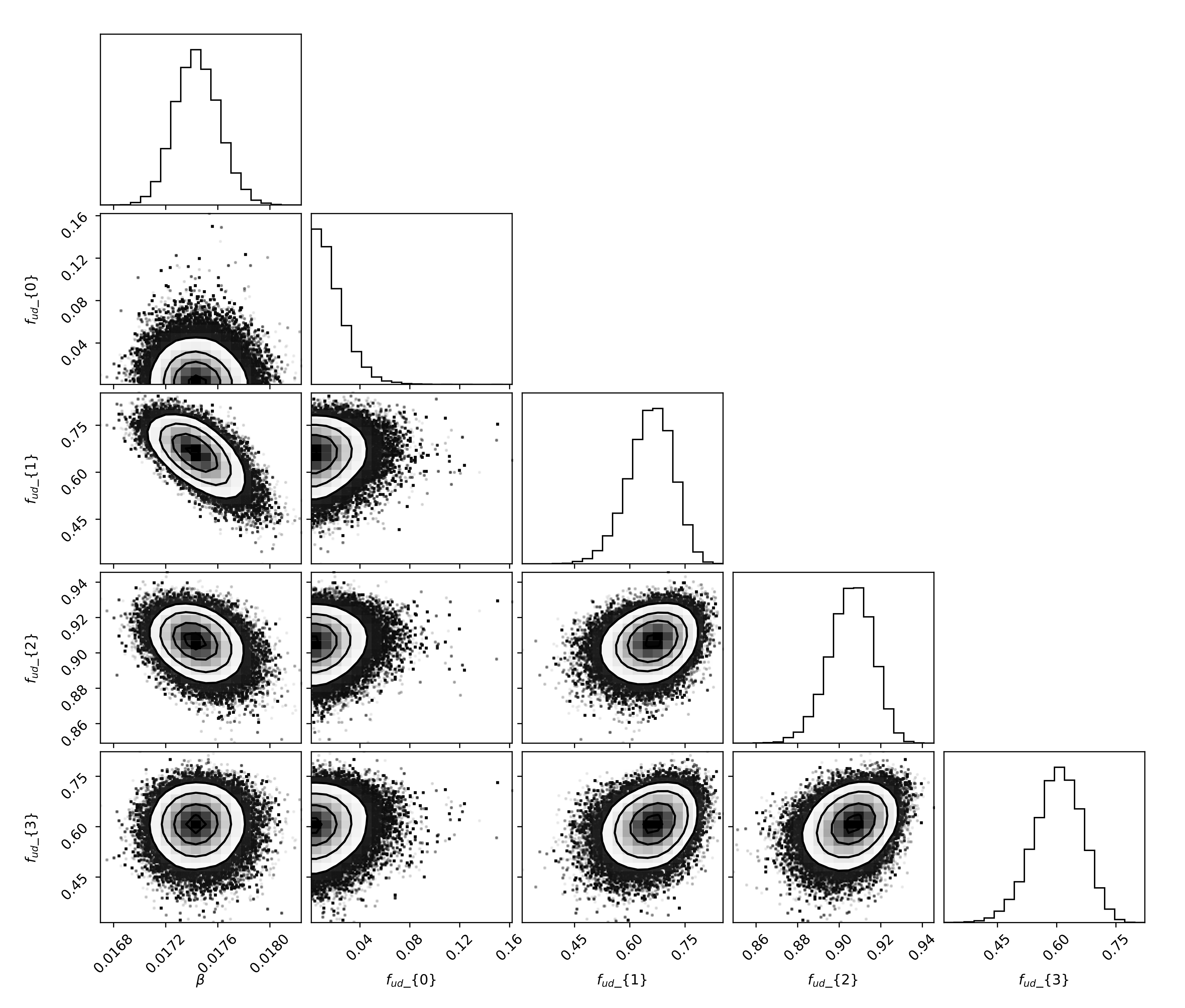
We’re now ready to generate our results, we’ll first calibrate the model using data up until January 1st, 2018. Then, we’ll increase the amount of available data until February 1st, 2018 and then March 1st, 2018, representing the moment right before, and right after, the peak incidence. Let’s first have a look at the sampled distributions of \(\beta\) and \(\mathbf{f_{ud}}\) on the largest dataset (ending March 1st, 2018).

The optimal values of the fraction of undetected cases \(\mathbf{f_{ud}}\) are: f_ud = [0.01, 0.64, 0.90, 0.60]. The undetected fraction is thus very small in children aged five years and below, then increases to 90% in individuals aged 15 to 65 years old, and finally decreases to 60% in the senior population. The population average basic reproduction number was \(R_0 = 1.95 (95~\%\ CI: 1.91-1.98)\).

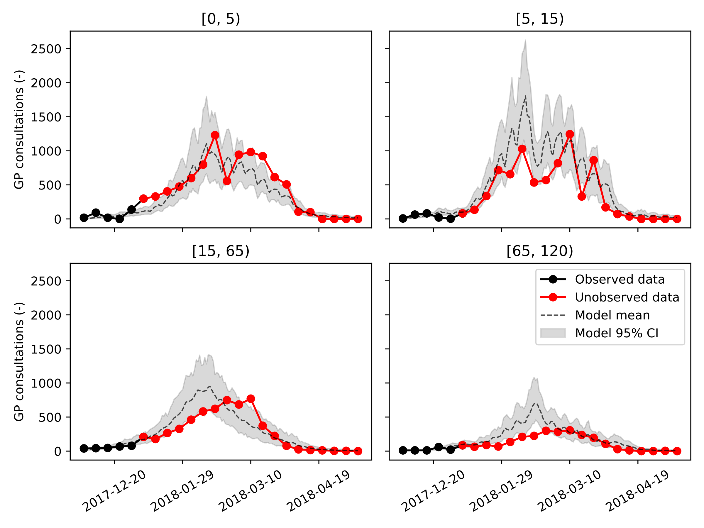
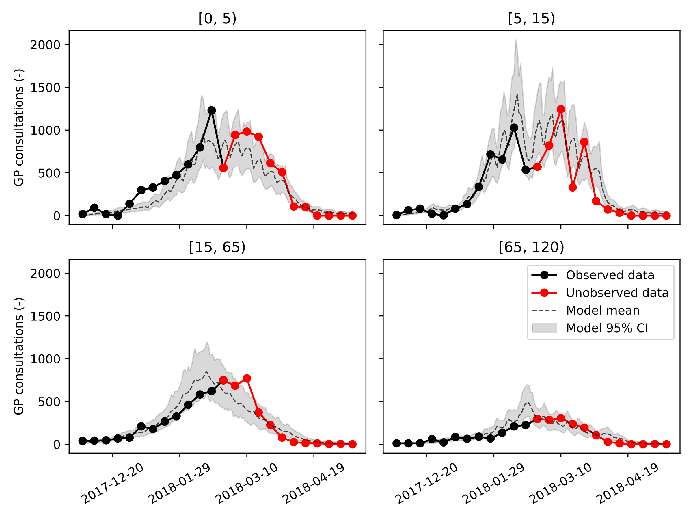
Next, we show, for every age group and for our three calibration datasets, the model trajectories plotted on top of the data. Considering how rudimentary this model is, even the predictions made on January 1st, 2018, one month and a half before the peak incidence, are reasonably accurate and can be informative to policymakers. It should be noted that the peak incidence in the adult age groups falls at least two weeks earlier than was the case in real life.

The results obtained using our simple model are encouraging but not yet sufficiently accurate to advice policy makers and GPs. To improve the accuracy of our simple model, we see two possibilities. First, by making the model spatially-explicit, we include more heterogeneity in the model rendering predicted epidemic peaks more broad under the same number of social contacts. Second, including vaccines could likely further improve this model’s accuracy by lowering the peak incidence in the elderly population, as vaccine uptake was found to increase significantly in individuals above fifty years old. Finally, the consistency of the obtained parameter estimates, as well as the accuracy of the calibration procedure should be demonstrated across multiple influenza seasons. However, this is out of the scope as the aim of this work is merely to highlight our code’s ability to speed up a modeling and simulation workflow.

Calibration ending on January 1st, 2018

Calibration ending on February 1st, 2018

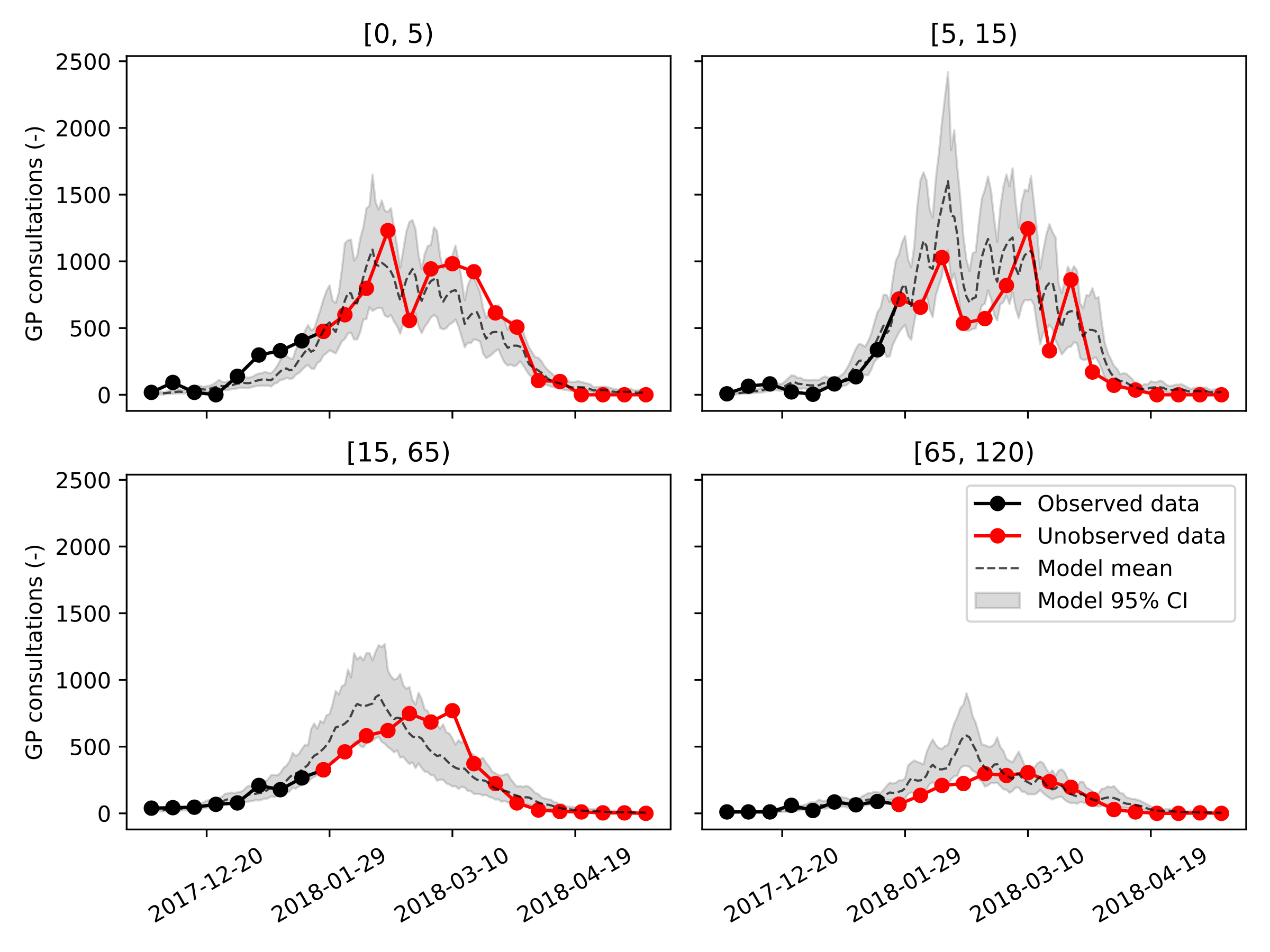
Calibration ending on March 1st, 2018