Modeling and Calibration Workflow
In this tutorial, we’ll use the simple SIR disease model without dimensions from the quickstart tutorial and calibrate its basic reproduction number to a synthetically generated dataset. We’ll then asses what happens if the pathogen’s infectivity is lowered by means of preventive measures. This tutorial steps you through a typical workflow constituting the following steps,
Import dependencies
Load the dataset
Define a pySODM model
Initialize the model
Calibrate the model (PSO/NM + MCMC)
Visualize the goodness-of-fit
Perform a scenario analysis
By using a simple model, we can focus on the general workflow and on the most important functions of pySODM, which will be similar in the more advanced enzyme kinetics and Influenza case studies available on this documentation website. This tutorial can be reproduced by running ~/tutorials/SIR/workflow_tutorial.py, an environment containing the dependencies needed to run this tutorial is provided in ~/tutorial_env.yml.
Import dependencies
I typically place all my dependencies together at the top of my script. However, for this demo, we’ll import some common dependencies here and then import the pySODM code on the go. That way, the imports of the necessary pySODM code are located where they are required which is more illustrative than including them all here at once.
import numpy as np
import pandas as pd
import matplotlib.pyplot as plt
Load the dataset
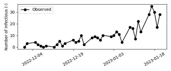
For the purpose of this tutorial, we’ll generate a sythetic dataset containing disease incidence. We assume the disease is generating cases exponentially with a doubling time of 10 days. Mathematically,
We’ll assume the first case was detected on December 1st, 2022 and data was collected on weekdays only until December 21st, 2022. Then, we’ll add observational noise to the synthetic data. For count based data, observational noise is typically the result of a poisson or negative binomial proces, depending on the occurence of overdispersion. In case the observations result from a poisson proces, the variance in the data is equal to the mean: \(\sigma^2 = \mu\), while for a negative binomial proces the mean-variance relationship is quadratic: \(\sigma^2 = \mu + \alpha \mu^2\). For this example we’ll use the negative binomial distribution with a dispersion factor of alpha=0.03, which was representative for the data used during the COVID-19 pandemic in Belgium. Note that for \(\alpha=0\), the variance of the negative binomial distribution is equal to the variance of the poisson distribution.
# Parameters
alpha = 0.03    # Overdispersion
t_d = 10         # Exponential doubling time
# Sample data
dates = pd.date_range('2022-12-01','2023-01-21')
t = np.linspace(start=0, stop=len(dates)-1, num=len(dates))
y = np.random.negative_binomial(1/alpha, (1/alpha)/(np.exp(t*np.log(2)/t_d) + (1/alpha)))
# Place in a pd.Series
d = pd.Series(index=dates, data=y, name='CASES')
# Index name must be date for calibration to work
d.index.name = 'date'
# Only retain weekdays
d = d[d.index.dayofweek < 5]
Datasets used in an optimization must always be a pd.Series, in case the model has no dimensions, or a pd.DataFrame with a pd.MultiIndex if the model has dimensions. In the dataset, an index level named time (if the time axis consists of int/float) or date (if the time axis consists of dates) must always be present. In this tutorial, we’ll use dates and thus we rename the index of our dataset date.
# Index name must be data for calibration to work
d.index.name = 'date'
print(d)
date
2022-12-01     1
2022-12-02     1
...
2023-01-19    34
2023-01-20    24
Name: CASES, dtype: int64
Visually,
Define and initialize the model
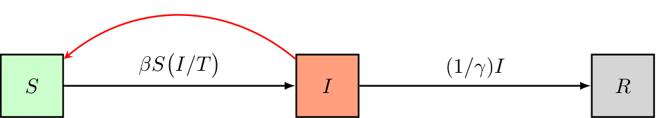
As an example, we’ll set up a simple Susceptible-Infectious-Removed (SIR) disease model, schematically represented as follows,
and governed by the following equations,
The model has three states: 1) The number of individuals susceptible to the disease (S), 2) the number of infectious individuals (I), and 3) the number of removed individuals (R). The model has two parameters: 1) beta, the rate of transmission and, 2) gamma, the duration of infectiousness. Building a pySODM model is based on class inheritance, you load the ODE class from ~/src/models/base.by. Then, you define your own model class which must contain (minimally),
A list containing the state names, named
states,A list containing the parameter names, named
parameter_names,A function named
integrate()where you compute your model’s differentials.
This class takes pySODM’s ODE class as its input. The ODE class is recognizes the components of your custom model class which will aid in performing input checks. Checkout the documentation of the ODE class for an overview of the class methods. There are some important formatting requirements to the integrate function, which are verified when the model is initialized,
The integrate function must have the timestep
tas its first inputFollowed by all model states and parameters, their order does not matter
The integrate function must return a differential for every model state, arranged in the same order as the state names defined in
statesThe integrate function must be a static method (done by decorating with
@staticmethod)
# Import the ODE class
from pySODM.models.base import ODE

# Define the model equations
class ODE_SIR(ODE):
    """
    An SIR model
    """

    states = ['S','I','R']
    parameters = ['beta','gamma']

    @staticmethod
    def integrate(t, S, I, R, beta, gamma):

        # Calculate total population
        N = S+I+R
        # Calculate differentials
        dS = -beta*S*I/N
        dI = beta*S*I/N - 1/gamma*I
        dR = 1/gamma*I

        return dS, dI, dR
After defining our model, we’ll initialize it by supplying a dictionary of initial states and a dictionary of model parameters. In this example, we’ll assume the disease spreads in a relatively small population of 1000 individuals. At the start of the simulation we’ll assume there is one “patient zero”. There’s no need to define the number of recovered individuals as undefined states are automatically set to zero by pySODM.
model = ODE_SIR(initial_states={'S': 1000, 'I': 1}, parameters={'beta': 0.35, 'gamma': 5})
Calibrating the model
The posterior probability function
Before we can have our computer find a set of model parameters that aligns the model with the data, we must instruct it what deviations between the data and model prediction are tolerated. Such function is often referred to as an objective function or likelihood function. In all tutorials we will set up and attempt to maximize the posterior probability of our model’s simulations in light of the data \(p(\tilde{x}(\theta) | x)\), which is mathematically defined as, $$ p (\tilde{x}(\theta) | x) = \frac{p( x | \tilde{x}(\theta)) p(\theta)}{p(x)}, $$ where \(x\) represents the data, \(\theta\) the model’s parameters, and \(\tilde{x}(\theta)\) a model simulation made using parameters \(\theta\). \(p(x | \tilde{x}(\theta))\) is the likelihood function, \(p(\theta)\) is the prior probability of the model parameters and contains any prior beliefs about the probability density distribution of the parameters \(\theta\). Finally, \(p(x)\) is the probability of the data, which is used for normalization and can be ignored for all practical purposes. What is therefore important to remember is that the posterior probability is proportional to the product of the likelihood and the parameter prior probability. We’ll maximize the logarithm of the posterior probability, which can be computed as the sum of the logarithm of the prior probability and the logarithm of the likelihood. Therefore,
$$\log p (\tilde{x}(\theta) | x) \propto \log p( x | \tilde{x}(\theta)) + \log p(\theta)$$
Just remember: LOG POSTERIOR = LOG PRIOR + LOG LIKELIHOOD
For an introduction to Bayesian inference, I recommend reading the following article. I also recommend going through the following tutorial of emcee.
Choosing an appropriate prior function
For every model parameter you calibrate, a probability function expressing our prior believes with regard to the probability distribution of that parameter must be provided. pySODM includes uniform, triangular, normal, gamma and beta priors, which can be imported as follows,
from pySODM.optimization.objective_functions import log_prior_uniform, log_prior_triangle, log_prior_normal, log_prior_gamma, log_prior_beta
When initializing the log_posterior probability class it is not necessary to define priors for your parameters (arguments log_prior_prob_fnc and log_prior_prob_fnc_args). If no priors are defined, by default, pySODM will initialize uniform priors for the calibrated parameters. For most problems, uniform prior probabilities – which simply constraint the parameter values within certain bounds – suffice.
Choosing an appropriate likelihood function
The next step is to choose an appropriate log likelihood function. The log likelihood function is a function that describes the magnitude of the error when model prediction and data deviate. The bread and butter log likelihood function is the sum of squared errors (SSE),
which is a simplified case of a normal log likelihood function,
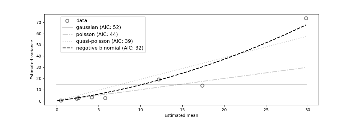
The normal log likelihood reduces to the SSE when the error on all datapoints are the same (i.e. \(\sigma_i^2 = 1\)), in technical terms, the SSE assumes the data are homoskedastic which is rarely the case in practice. If the errors (\(\sigma_i\)) of all datapoints (\(y_{data,i}\)) are known, then the normal log likelihood function is the maximum likelihood estimator. When the error of the datapoints are unknown, we can analyze the relationship between the magnitude of the data and its variance to help us choose the most appropriate likelihood function. For epidemiological case data, only one datapoint is available per day implying no error is readily available. However, in count data dispersion tends to increase linearily with the magnitude of the data. In that case, pySODM’s variance_analysis() function includes a functionality to approximate the mean-variance relationship in a dataset of counts. To do so, we assume a moving exponential average of the data accurately represents the underlying undispersed truth, we then dividing the data in discrete windows, and then compute the dispersion of the data around the exponential moving average’s mean within every window to obtain mean-variance couples. Then, the appropriate likelihood function can be found by fitting the following candidate mean-variance relationships,
Mean-Variance model |
Relationship |
|---|---|
Gaussian |
\(\sigma^2 = c\) |
Poisson |
\(\sigma^2 = \mu\) |
Quasi-Poisson |
\(\sigma^2 = \alpha * \mu\) |
Negative Binomial |
\(\sigma^2 = \mu + \alpha * \mu^2\) |
For a more rigorous explanation of the procedure, we highly recommend reading section E.1 in the Supplementary Materials of this article. The following code snippet performs the estimation for our synthetic dataset.
from pySODM.optimization.utils import variance_analysis

results, ax = variance_analysis(d, window_length='W', half_life=3.5)
alpha = results.loc['negative binomial', 'theta']
print(results)
plt.show()
plt.close()
                       theta        AIC
gaussian           14.568640  52.300657
poisson             0.000000  44.165044
quasi-poisson       1.925682  38.796586
negative binomial   0.042804  32.045864
The negative binomial model with dispersion coefficient \(\alpha = 0.043\) is the most appropriate statistical model (lowest AIC). This estimate is quite good considering we’re using a very limited amount of data generated from a negative binomial model with a dispersion coefficient \(\alpha = 0.03\). We highly recommend varying both the window size and the length of the exponential filter before committing to any likelihood function.
Setting up the posterior probability in pySODM
Let’s initialize an appropriate posterior probability function for the problem at hand. We start by importing the log_posterior_probability class and the negative binomial likelihood function ll_negative_binomial. The following arguments of log_posterior_probability are mandatory,
model: The previously initialized model.pars: A list containing the names of the model parameters we wish to optimize. pySODM can be used to calibrate 0D, 1D and nD model parameters.bounds: A list containing the lower and an upper bounds of the parameters.data: A list containing the datasets we wish to calibrate our model to.states: A list containing, for every dataset, the model state that must be matched with it.log_likelihood_function: A list containing, for every dataset, the log likelihood function used to describe deviations between the model prediction and the respective dataset.log_likelihood_function_args: A list containing the arguments of every log likelihood function.
The lengths of the number of data, states, log_likelihood function and log_likelihood_function_args must always be equal. In the example, as no prior functions are provided, the priors will default to uniform priors over the provided bounds. Providing a label is also optional, if no label is provided, the names provided in pars are used as labels.
if __name__ == '__main__':

    # Import the log_posterior_probability class
    from pySODM.optimization.objective_functions import log_posterior_probability

    # Import the negative binomial likelihood function
    from pySODM.optimization.objective_functions import ll_negative_binomial

    # The datasets, the model states to match to the datasets,
    # the log likelihood functions and log likelihood function arguments
    data=[d, ]
    states = ["I",]
    log_likelihood_fnc = [ll_negative_binomial,]
    log_likelihood_fnc_args = [alpha,]

    # Calibated parameters, their bounds and preferred labels
    pars = ['beta',]
    bounds = [(1e-6,1),]
    labels = ['$\\beta$',]

    # Setup objective function
    # (no priors --> uniform priors based on bounds)
    objective_function = log_posterior_probability(model, pars, bounds, data, states, log_likelihood_fnc, log_likelihood_fnc_args, labels=labels)
If we wanted to use a normal prior distribution for beta,
# Import the normal prior probability distribution
from pySODM.optimization.objective_functions import log_prior_normal

# Define the additional arguments of the log_posterior_probability class
log_prior_prob_fnc = [log_prior_normal,]
log_prior_prob_func_args = [{'avg': 0.3, 'stdev': 0.1},]

# Setup objective function
objective_function = log_posterior_probability(model, pars, bounds, data, states, log_likelihood_fnc, log_likelihood_fnc_args, log_prior_prob_fnc, log_prior_prob_func_args, labels=labels)
Nelder-Mead optimization
The following code snippet starts a Nelder-Mead optimization from the initial guess \(\beta = 0.35\), perturbated with a step of 10%. Running on processes=1 cores for max_iter=10 iterations.
if __name__ == '__main__':
    # Import the Nelder-Mead algorithm
    from pySODM.optimization import nelder_mead
    # Initial guess
    theta = [0.35,]
    # Run Nelder-Mead optimisation
    theta, _ = nelder_mead.optimize(objective_function, theta, step=[0.10,], processes=1, max_iter=10)
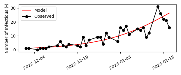
We find an optimal value of \(\beta \pm 0.27\). We can then asses the goodness-of-fit by updating the dictionary of model parameters with the newly found value for beta, simulating the model and visualizing the model prediction and dataset.
if __name__ == '__main__':
    # Update beta with the calibrated value
    model.parameters.update({'beta': theta[0]})
    # Simulate the model
    out = model.sim([d.index.min(), d,index.max()])
    # Visualize result
    fig,ax=plt.subplots()
    ax.plot(out['date'], out['I'], color='red', label='Infectious')
    ax.scatter(d.index, d.values, color='black', alpha=0.6, linestyle='None', facecolors='none', s=60, linewidth=2, label='data')
    ax.legend()
    plt.show()
    plt.close()
Quite nice!
Bayesian inference
This approach moves away from the idea of accepting a single parameter value being the best fit to the data, and instead identifies all regions of the parameter space that are in agreement with the observations. In the language of Bayesian inference, what we seek is called the posterior distribution of the parameters: a probability distribution on the parameter space that assigns higher probability to areas that are in better agreement with the observations. Here, we demonstrate that a Bayesian approach provides accurate estimates of model parameters and their uncertainty.
We’ll use our previous estimate to initiate our Markov-Chain Monte-Carlo sampler. This requires the help of two functions: perturbate_theta() and run_EnsembleSampler(). We’ll initiate 9 chains per calibrated parameter, so there will be 9 chains in total. To do so, we’ll first use perturbate_theta to perturbate our previously obtained estimate theta by 10%. The result is a np.ndarray pos of shape (1, 9), which we’ll then pass on to run_EnsembleSampler().
Then, we’ll setup and run the sampler using run_EnsembleSampler() until the chains converge. We’ll run the sampler for n_mcmc=100 iterations and print the diagnostic autocorrelation and trace plots every print_n=10 iterations in a folder called sampler_output/. For convenience, a copy of the samples is saved in an xarray.Dataset as well every print_n=10 iterations. As an identifier for our experiment, we’ll use 'username'. While the sampler is running, have a look in the sampler_output/ folder, which should look as follows,
├── sampler_output
|   |── username_BACKEND_YYYY-MM-DD.hdf5
|   |── username_SAMPLES_YYYY-MM-DD.nc
|   |── username_AUTOCORR_YYYY-MM-DD.pdf
│   └── username_TRACE_YYYY-MM-DD.pdf
The first output of run_EnsembleSampler() is an emcee.EnsembleSampler object containing our 100 iterations for 9 chains. We can extract the samples manually by using its get_chain() method, along with many more emcee related operations (see the emcee documentation). However, we’re interested in the second output of run_EnsembleSampler(), which contains the samples in an xarray.Dataset, indexed on the chain and iteration numbers. This interfaces nicely to pySODM’s draw functions (introduced below). Finally, we’ll use the third-party corner package to visualize the distributions of the five calibrated parameters.
if __name__ == '__main__':

    from pySODM.optimization.mcmc import perturbate_theta, run_EnsembleSampler
    # Settings
    n_mcmc = 100
    multiplier_mcmc = 9
    processes = 9
    print_n = 10
    discard = 20
    samples_path = 'sampler_output/'
    fig_path = 'sampler_output/'
    identifier = 'username'
    # Perturbate previously obtained estimate
    ndim, nwalkers, pos = perturbate_theta(theta, pert=[0.10,], multiplier=multiplier_mcmc, bounds=bounds)
    # Usefull settings to retain in the samples dictionary (no pd.Timestamps or np.arrays allowed!)
    settings={'start_calibration': d.index.min().strftime("%Y-%m-%d"), 'end_calibration': end_date.strftime("%Y-%m-%d"), 'starting_estimate': list(theta)}
    # Run the sampler
    sampler, samples_xr = run_EnsembleSampler(pos, n_mcmc, identifier, objective_function, fig_path=fig_path, samples_path=samples_path, print_n=print_n, processes=processes, progress=True, settings_dict=settings)

    print(samples_xr)
The resulting xarray.Dataset contains the samples of beta, as well as the variables defined in the settings dictionary. It is identical to the samples automatically saved in sampler_output/username_SAMPLES_YYYY-MM-DD.nc.
<xarray.Dataset> Size: 24kB
Dimensions:    (iteration: 300, chain: 9)
Coordinates:
  * iteration  (iteration) int64 2kB 0 1 2 3 4 ... 296 297 298 299
  * chain      (chain) int64 72B 0 1 2 3 4 5 6 7 8
Data variables:
    beta       (iteration, chain) float64 22kB 0.2818 ... 0.2761
Attributes:
    start_calibration:  2022-12-01
    end_calibration:    2023-01-20
    starting_estimate:  [0.2764298804104327]
Results
Basic reproduction number
For our simple SIR model, the basic reproduction number is defined as,
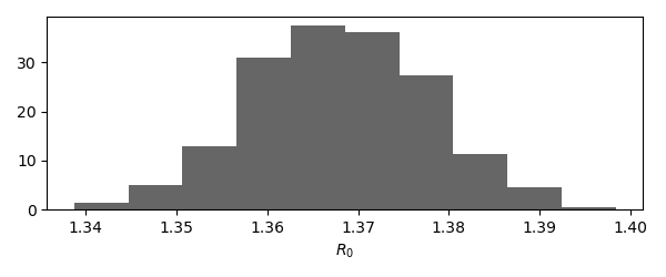
Using the obtained samples, we find a basic reproduction number of \(R_0 = 1.37 \pm 0.01\). Its distribution looks as follows,
# Visualize the distribution of the basic reproduction number
fig,ax=plt.subplots()
ax.hist(samples_xr['beta'].values.flatten()*model.parameters['gamma'], density=True, color='black', alpha=0.6)
ax.set_xlabel('$R_0$')
plt.show()
plt.close()
Goodness-of-fit: draw functions
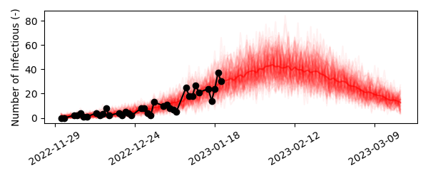
Next, let’s visualize how well our simple SIR model fits the data. To this end, we’ll simulate the model a number of times, and we’ll update the value of beta with a sample from its posterior probability distribution obtained using the MCMC. Then, we’ll add the noise introduced by observing the epidemiological process to each simulated model trajectory using add_negative_binomial(). Finally, we’ll visualize the individual model trajectories and the data to asses the goodness-of-fit.
To repeatedly simulate a model and update a parameter value in each consecutive run, you can use pySODM’s draw function. These functions always take the model parameters as its first input argument, followed by an arbitrary number of user-defined parameters to aid in the draw function. A draw function must always return the dictionary of model parameters, without alterations to the dictionaries keys. The draw function defines how parameters and initial conditions can change during consecutive simulations of the model, i.e. it updates parameter values in the model parameters dictionary. This feature is useful to perform sensitivty analysis.
In this example, we’ll use a draw function to replace beta with a random value obtained from its posterior probability distribution obtained during sampling. We accomplish this by defining a draw function with one additional argument, samples, which is a list containing the samples of the posterior probability distribution of beta. np.random.choice() is used to sample a random value of beta and assign it to the model parameteres dictionary,
# Define draw function
def draw_fcn(parameters, samples):
    parameters['beta'] = np.random.choice(samples)
    return parameters
To use this draw function, you provide four additional arguments to the sim() function,
N: the number of repeated simulations,draw_function: the draw function,draw_function_kwargs: a dictionary containing all parameters of the draw function not equal toparameters.processes: the number of cores to divide theNsimulations over.
As demonstrated in the quickstart example, the xarray.Dataset containing the model output will now contain an additional dimension to accomodate the repeated simulations: draws.
# Simulate model
out = model.sim([d.index.min(), d.index.max()+pd.Timedelta(days=28)], N=50, draw_function=draw_fcn, draw_function_kwargs={'samples': samples_xr['beta'].values.flatten()}, processes=processes)
# Add negative binomial observation noise
out = add_negative_binomial_noise(out, dispersion)
# Visualize result
fig,ax=plt.subplots(figsize=(12,4))
for i in range(30):
    ax.plot(out['date'], out['I'].isel(draws=i), color='red', alpha=0.05)
ax.plot(out['date'], out['I'].mean(dim='draws'), color='red', alpha=0.6)
ax.scatter(d.index, d.values, color='black', alpha=0.6, linestyle='None', facecolors='none', s=60, linewidth=2)
ax.xaxis.set_major_locator(plt.MaxNLocator(3))
plt.show()
plt.close()
Our simple SIR model fits the data well. From the projection we can deduce that the peak number of infectees will fall around February 7th, 2023 and there will be between 30-50 infectees.
Scenarios: time-dependent model parameters
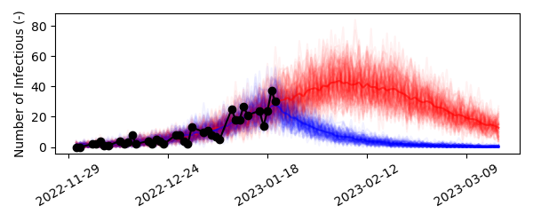
Finally, let us introduce the concept of varying model parameters over the course of the simulation. We would like to model what would happen if we could somehow reduce the infectivity of the disease by 50% starting January 21st. In the real world this could be accomplished by raising awareness to the disease and applying preventive measures.
We’ll first need to implement a function to let our model know how a given parameter should vary over time: a time-dependent model parameter function (TDPF). Then, we’ll need to re-initialize our model and tell it what model parameter should be varied in accordance to our function. For our problem, a TDPF would have the following syntax,
# Define a time-dependent parameter function
def lower_infectivity(t, states, param, start_measures):
    if t < start_measures:
        return param
    else:
        return 0.50*param
This simple function reduces the parameter param with a factor two if the simulation date is larger than start_measures. A time-dependent model parameter function must always have the arguments t (simulation timestep), states (dictionary of model states) and param (original value of the parameter the function is applied to) as inputs. In addition, the user can supply additional arguments to the function, which need to be added to the dictionary of model parameters when the model is initialised.
We will apply this function to the infectivity parameter beta, and declare this using the time_dependent_parameters argument when initialising the model.
# Attach the additional arguments of the time-depenent function to the parameter dictionary
model.parameters.update({'start_measures': '2023-01-21'})

# Initialize the model with the time dependent parameter funtion
model_with = ODE_SIR(initial_states=init_states, parameters=model.parameters,
                     time_dependent_parameters={'beta': lower_infectivity})
Next, we compare the simulations with and without the use of our time-dependent model parameter function.
# Simulate the model
out_with = model_with.sim([d.index.min(), d.index.max()+pd.Timedelta(days=2*28)], N=50, draw_function=draw_fcn, draw_function_kwargs={'samples': samples_xr['beta'].values.flatten()} processes=processes)

# Add negative binomial observation noise
out_with = add_negative_binomial_noise(out_with, alpha)

# Visualize result
fig,ax=plt.subplots(figsize=(12,4))
for i in range(50):
    ax.plot(out['date'], out['I'].isel(draws=i), color='red', alpha=0.05)
    ax.plot(out_with['date'], out_with['I'].isel(draws=i), color='blue', alpha=0.05)
ax.plot(out['date'], out['I'].mean(dim='draws'), color='red', alpha=0.6)
ax.plot(out_with['date'], out_with['I'].mean(dim='draws'), color='blue', alpha=0.6)
ax.scatter(d.index, d.values, color='black', alpha=0.6, linestyle='None', facecolors='none', s=60, linewidth=2)
ax.xaxis.set_major_locator(plt.MaxNLocator(3))
ax.set_ylabel('Number of infected')
plt.show()
plt.close()
As we could reasonably expect, if we could implement some form of preventive measures on January 21st that slashes the infectivity in half, cases quite abruptly start declining and thus less people contrapt the disease.
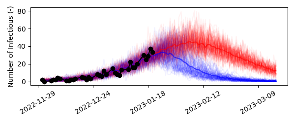
However, it is unlikely that people would adopt these preventive measures instantly. Adoptation of measures is more gradual in the real world. We could tackle this problem in two ways using pySODM,
Implementing a ramp function to gradually lower the infectivity in our time-dependent model parameter function,
Using draw functions to sample
start_measuresstochastically in every simulation. We’ll demonstrate this option.
To simulate ramp-like adoptation of measures, we can add the number of additional days it takes beyond January 21st, 2023 to adopt the measures by sampling from a triangular distribution with a minimum and mode of zero days, and a maximum adoptation time of ramp_length days. All we have to do is add one line to the draw function,
# Define draw function
def draw_fcn(parameters, samples, ramp_length):
    parameters['beta'] = np.random.choice(samples)
    parameters['start_measures'] += pd.Timedelta(days=np.random.triangular(left=0,mode=0,right=ramp_length))
    return parameters
Don’t forget to add the new parameter ramp_length to the dictionary of draw_function_kwargs when simulating the model! Gradually adopting the preventive measures results in a more realistic simulation,
Conclusion
I hope this tutorial has demonstrated a simple yet common workflow pySODM can speedup for you. However, both our model and dataset had no labeled dimensions (0-dimensional) so this example was very rudimentary. However, pySODM allows to tackle higher-dimensional problems using the same basic syntax. This allows to tackle complex problems in different scientific disciplines, I illustrate this with the following tutorials,
Case study |
Features |
|---|---|
Enzyme kinetics: intrinsic kinetics |
Calibration of a model to multiple datasets with changing initial conditions. |
Enzyme kinetics: 1D Plug-Flow Reactor |
Use the method of lines to discretise a PDE model into an ODE model and simulate it using pySODM. |
Influenza 2017-2018 |
Stochastic jump process epidemiological model with age groups (1D model). Calibration of a 1D model parameter to a 1D dataset. |
SIR-SI Model |
ODE model where states have different dimensions and thus different shapes. |