Quickstart
Set up a dimensionless ODE model
To set up a simple Susceptible-Infectious-Removed (SIR) disease model, schematically represented as follows,
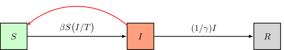
and governed by the following equations,
Load pySODM’s ODE class, and then define your model class–inheriting pySODM’s ODE class–to define your model. Minimally, you must provide: 1) A list containing the names of your model’s states, 2) a list containing the names of your model’s parameters, 3) an integrate function integrating your model’s states. To learn more about the ODE class’ formatting, check out the ODE class description.
# Import the ODE class
from pySODM.models.base import ODE

# Define the model equations
class SIR(ODE):

    states = ['S','I','R']
    parameters = ['beta','gamma']

    @staticmethod
    def integrate(t, S, I, R, beta, gamma):

        # Calculate total population
        N = S+I+R
        # Calculate differentials
        dS = -beta*S*I/N
        dI = beta*S*I/N - 1/gamma*I
        dR = 1/gamma*I

        return dS, dI, dR
To initialize the model, provide a dictionary containing the initial condition and a dictionary containing all model parameters. Undefined initial states are automatically filled with zeros.
model = SIR(initial_states={'S': 1000, 'I': 1}, parameters={'beta': 0.35, 'gamma': 5})
Alternatively, use an initial condition function to define the initial states,
# can have arguments
def initial_condition_function(S0):
    return {'S': S0, 'I': 1}

# that become part of the model's parameters and can be optimised..
model = SIR(initial_states=initial_condition_function, parameters={'beta': 0.35, 'gamma': 5, 'S0': 1000})
Simulate the model using its sim() method. pySODM supports the use of dates to index simulations, string representations of dates with the format 'yyyy-mm-dd' as well as datetime.datetime() can be used to define the start- and enddate of a simulation. By default, pySODM assumes the unit of time is days, but you can change this using the time_unit input.
# Timesteps
out = model.sim(121)

# String representation of dates:
# 'yyyy-mm-dd' only (no hours, min, seconds -> use datetime)
out = model.sim(['2022-12-01', '2023-05-01'])

# Datetime representation of time + date
# A timestep of length 1 represents one week
from datetime import datetime as datetime
out = model.sim([datetime(2022, 12, 1), datetime(2023, 5, 1)], time_unit='W')

# Tailor method and tolerance of integrator
out = model.sim(121, method='RK45', rtol='1e-4')
In some situations, the use of a discrete timestep with a fixed length may be preferred,
out = model.sim(121, tau=1) # Use a discrete timestepper with step size 1
Simulations are sent to an xarray.Dataset, for more information on indexing and selecting data using xarray, see.
<xarray.Dataset>
Dimensions:  (time: 122)
Coordinates:
  * time     (time) int64 0 1 2 3 4 5 6 7 8 ... 114 115 116 117 118 119 120 121
Data variables:
    S        (time) float64 1e+03 999.6 999.2 998.7 ... 287.2 287.2 287.2 287.2
    I        (time) float64 1.0 1.161 1.348 1.565 ... 0.1455 0.1316 0.1192
    R        (time) float64 0.0 0.2157 0.4662 0.7569 ... 713.6 713.7 713.7 713.7
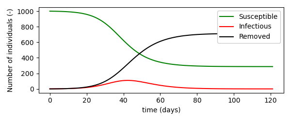
The simulation above results in the following trajectories for the number of susceptibles, infected and recovered individuals.
Set up an ODE model with a labeled dimension
To transform all our SIR model’s states in 1D vectors, referred to as a dimension throughout the documentation, add the dimensions keyword to the model declaration. In the example below, we add a dimension representing the age groups individuals belong to. This turns all model states in the integrate function into 1D vectors.
# Import the ODE class
from pySODM.models.base import ODE

# Define the model equations
class stratified_SIR(ODE):

    states = ['S','I','R']
    parameters = ['beta', 'gamma']
    dimensions = ['age_groups']

    @staticmethod
    def integrate(t, S, I, R, beta, gamma):

        # Calculate total population
        N = S+I+R
        # Calculate differentials
        dS = -beta*S*I/N
        dI = beta*S*I/N - 1/gamma*I
        dR = 1/gamma*I

        return dS, dI, dR
When initializing your model, provide a dictionary containing coordinates for every dimension declared previously. In the example below, we’ll declare four age groups: 0-5, 5-15, 15-65 and 65-120 year olds. All model states are now 1D vectors of shape (4,).
model = stratified_SIR(initial_states={'S': 1000*np.ones(4), 'I': np.ones(4)},
                       parameters={'beta': 0.35, 'gamma': 5},
                       coordinates={'age_groups': ['0-5','5-15', '15-65','65-120']})
out = model.sim(121)
print(out)
The dimension 'age_groups' with coordinates ['0-5','5-15', '15-65','65-120'] is automatically added to the model output.
<xarray.Dataset>
Dimensions:     (time: 122, age_groups: 4)
Coordinates:
  * time        (time) int64 0 1 2 3 4 5 6 7 ... 114 115 116 117 118 119 120 121
  * age_groups  (age_groups) <U6 '0-5' '5-15' '15-65' '65-120'
Data variables:
    S           (age_groups, time) float64 1e+03 999.6 999.2 ... 287.2 287.2
    I           (age_groups, time) float64 1.0 1.161 1.348 ... 0.1316 0.1192
    R           (age_groups, time) float64 0.0 0.2157 0.4662 ... 713.7 713.7
Set up an ODE model with multiple dimensions
pySODM allows model states to have different coordinates and thus different sizes. As an example (without mathematical details), consider an extension of the SIR model for vector borne disease: the SIR-SI model. In the example, the S, I and R states represent the humans, and we use the dimensions_per_state variable to declare the humans are distributed in four age groups. The S_v and I_v states represent the vectors and infected vectors are able to transmit a disease to the humans. In turn, infected humans can pass the disease back to the vector (see flowchart). Because in some contexts having age groups for our vectors is not relevant (f.i. mosquitos), we thus assign no dimensions to the S_v and I_v states.
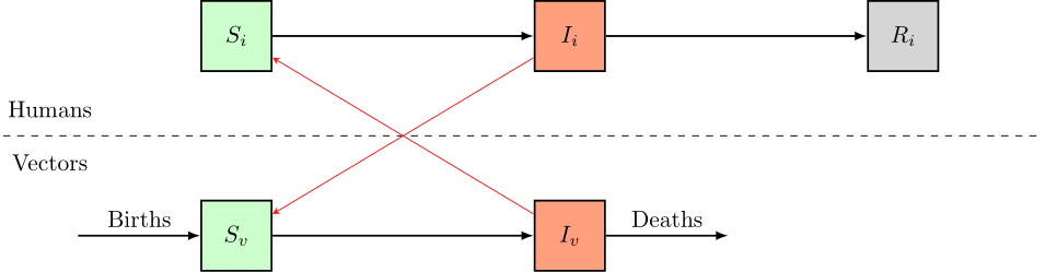
In the example below, the states S, I and R will be 1D vectors in the integrate function, while the states S_v and I_v will be scalars.
class ODE_SIR_SI(ODE):
    """
    An age-stratified SIR model for humans, an unstratified SI model for a disease vector (f.i. mosquito)
    """

    states = ['S', 'I', 'R', 'S_v', 'I_v']
    parameters = ['beta', 'gamma']
    stratified_parameters = ['alpha']
    dimensions = ['age_group']
    dimensions_per_state = [['age_group'],['age_group'],['age_group'],[],[]]

    @staticmethod
    def integrate(t, S, I, R, S_v, I_v, alpha, beta, gamma):

        # Calculate total mosquito population
        N = S + I + R
        N_v = S_v + I_v
        # Calculate human differentials
        dS = -alpha*(I_v/N_v)*S
        dI = alpha*(I_v/N_v)*S - 1/gamma*I
        dR = 1/gamma*I
        # Calculate mosquito differentials
        dS_v = -np.sum(alpha*(I/N)*S_v) + (1/beta)*N_v - (1/beta)*S_v
        dI_v = np.sum(alpha*(I/N)*S_v) - (1/beta)*I_v

        return dS, dI, dR, dS_v, dI_v
Setting up and simulating the model,
# Define parameters, initial states and coordinates
params={'alpha': np.array([0.05, 0.1, 0.2, 0.15]), 'gamma': 5, 'beta': 7}
init_states = {'S': [606938, 1328733, 7352492, 2204478], 'S_v': 1e6, 'I_v': 2}
coordinates={'age_group': ['0-5','5-15', '15-65','65-120']}
# Initialize model
model = ODE_SIR_SI(initial_states=init_states, parameters=params, coordinates=coordinates)
# Simulate the model
out = model.sim(120)
print(out)
results in the following xarray.Dataset,
<xarray.Dataset>
Dimensions:    (age_group: 4, time: 121)
Coordinates:
  * age_group  (age_groups) <U6 '0-5' '5-15' '15-65' '65-120'
  * time       (time) int64 0 1 2 3 4 5 6 7 ... 113 114 115 116 117 118 119 120
Data variables:
    S          (age_group, time) float64 6.069e+05 6.069e+05 ... 1.653e+06
    I          (age_group, time) float64 0.0 0.05178 ... 1.4e+05 1.464e+05
    R          (age_group, time) float64 0.0 0.00545 ... 3.76e+05 4.047e+05
    S_v        (time) float64 1e+06 1e+06 1e+06 ... 8.635e+05 8.562e+05
    I_v        (time) float64 2.0 1.798 1.725 ... 1.292e+05 1.365e+05 1.438e+05
Here, S, I and R state have age_group and time as dimensions and their shape is thus (4,), while S_v and I_v only have time as dimension and their shape is thus (1,).
Set up a dimensionless stochastic jump process Model
To stochastically simulate the simple SIR model, pySODM’s JumpProcess class is loaded and two functions, compute_rates and apply_transitionings, must be defined instead of one. For a detailed mathematical description of implenting models using Gillespie’s tau-leaping method (example of a jump proces), we refer to the peer-reviewed paper. The rates dictionary defined in compute_rates contains the rates of the possible transitionings in the system. These are contained within a list so that a state may have multiple transitionings. To learn more about the JumpProcess class’ formatting, check out the JumpProcess class description.
# Import the ODE class
from pySODM.models.base import JumpProcess

# Define the model equations
class SIR(JumpProcess):

    states = ['S','I','R']
    parameters = ['beta','gamma']

    @staticmethod
    def compute_rates(t, S, I, R, beta, gamma):

        # Calculate total population
        N = S+I+R
        # Compute rates per model state
        rates = {
            'S': [np.array(beta*(I/N)),],
            'I': [np.array(1/gamma)],
        }
        return rates

    @staticmethod
    def apply_transitionings(t, tau, transitionings, S, I, R, beta, gamma):

        S_new  = S - transitionings['S'][0]
        I_new = I + transitionings['S'][0] - transitionings['I'][0]
        R_new = R + transitionings['I'][0]

        return S_new, I_new, R_new
Advanced simulation features
Draw functions
The simulation functions of the ODE and JumpProcess classes can be used to perform \(N\) repeated simulations by using the optional argument N. A draw function can be used to instruct the alteration of model parameters during consecutive model runs, thereby offering a powerful tool for sensitivity analysis and uncertainty propagation.
Draw functions always take the dictionary of model parameters as their first argument. This can be followed an arbitrary number of user-defined parameters, which must be supplied to the sim() function through the draw_function_kwargs argument. The output of a draw function is always the dictionary of model parameters, without alterations to the dictionaries keys (no new or removed parameters). In the example below, we attempt to draw a model parameter gamma randomly in the range [0, 5],
# make an example of a dictionary containing samples of a parameter `gamma`
samples = np.random.uniform(low=0, high=5, n=100)

# define a 'draw function'
def draw_function(parameters, samples):
    """ randomly selects a sample of 'gamma' from the provided dictionary of `samples` and
        assigns it to the dictionary of model `parameters`
    """
    parameters['gamma'] = np.random.choice(samples)
    return parameters

# simulate 10 trajectories, exploit 10 cores to speed up the computation
out = model.sim(121, N=10, draw_function=draw_function, draw_function_kwargs={'samples': samples}, processes=10)
print(out)
An additional dimension 'draws' will be added to the xarray.Dataset to accomodate the results of the repeated simulations.
<xarray.Dataset>
Dimensions:     (time: 122, age_groups: 4, draws: 10)
Coordinates:
  * time        (time) int64 0 1 2 3 4 5 6 7 ... 114 115 116 117 118 119 120 121
  * age_groups  (age_groups) <U6 '0-5' '5-15' '15-65' '65-120'
Dimensions without coordinates: draws
Data variables:
    S           (draws, age_groups, time) float64 1e+03 999.6 ... 316.9 316.9
    I           (draws, age_groups, time) float64 1.0 1.007 ... 0.1644 0.1492
    R           (draws, age_groups, time) float64 0.0 0.3439 ... 684.0 684.0
This example can also be coded up by drawing the random samples of gamma within the draw function,
# define a 'draw function'
def draw_function(parameters):
    parameters['gamma'] = np.random.uniform(low=0, high=5)
    return parameters

# simulate the model
out = model.sim(121, N=10, draw_function=draw_function)
NOTE Internally, a call to draw_function is made within the sim() function, where it is given the dictionary of model parameters, followed by the draw_function_kwargs.
Time-dependent parameter functions
Parameters can also be varied through the course of one simulation using a time-dependent parameter function (TDPF), which can be an arbitrarily complex function. A time-dependent parameter function always has the current timestep (t), the dictionary containing the model states (states) at time t, and the original value of the parameter it is applied to (param) as its inputs. Additionally, the function can take any number of additional user-defined arguments (including other model parameters).
def vary_my_parameter(t, states, param, an_additional_parameter):
    """A function to implement a time-dependency on a parameter"""

    # Do any computation
    param = ...

    return param
When initialising the model, all we need to do is use the time_dependent_parameters keyword to declare what parameter our TDPF should be applied to. Additional parameters introduced in TDPFs, in this example an_additional_parameter, should be added to the parameters dictionary.
model = SIR(initial_states={'S': 1000, 'I': 1},
            parameters={'beta': 0.35, 'gamma': 5, 'an_additional_parameter': any_datatype_you_want},
            time_dependent_parameters={'beta': vary_my_parameter})